Control algorithms

Cost optimization

Voltmasters' price-based control algorithm: plan the battery around dynamic energy prices to minimize cost.

Cost optimization is Voltmasters' price-based control algorithm. It minimizes the energy cost of the installation by deciding, every control cycle, how to charge and discharge the battery, based on forecasted energy prices and forecasts of PV production and consumption.

How it works

Every control cycle the algorithm:

Looks ahead over the forecast horizon (the time window it looks ahead through) at the dynamic (day-ahead) prices, the expected PV production and the expected consumption.
Plans the battery so energy is stored when it is cheap (or from PV surplus) and used, or injected, when it is expensive. This forward plan is the battery schedule.
Only acts when it pays off: charging and discharging are planned only when the price difference is large enough to outweigh the battery's round-trip losses (a configurable minimum price difference).
Respects the limits: the battery's minimum and maximum state of charge (SoC) and the grid connection limits (maximum injection and consumption).

The detailed plan, the event types and a worked example are described on the Battery schedule page. The rest of this page explains how the algorithm reaches those decisions.

Two loops: planning and acting

Cost optimization runs as two cooperating loops that share one artefact: the battery schedule.

The planning loop looks at the whole forecast horizon and works out the cheapest charge/discharge plan. It makes the plan. The plan is recomputed regularly, at every new 15-minute slot and whenever a fresh forecast arrives, so it always reflects the latest prices, production and the real battery state.
The control loop runs every control cycle (about once per second). It reads the single schedule entry that covers now, turns it into concrete setpoints (target values) for battery, PV and EV, and adapts those to live measurements and limits. It carries the plan out.

flowchart LR
    subgraph inputs["Forecasts and live state"]
        P["Day-ahead prices"]
        PV["PV production forecast"]
        C["Consumption forecast"]
        B["Battery state of charge"]
    end

    GEN["Generate battery schedule<br/>planning loop"]
    SCHED[("Battery schedule")]
    READ["Read entry for now<br/>control loop, approx 1s"]
    SET["Translate to battery / PV / EV setpoints"]
    HW["Battery, PV, grid connection"]

    P --> GEN
    PV --> GEN
    C --> GEN
    B --> GEN
    GEN --> SCHED
    SCHED --> READ
    READ --> SET
    SET --> HW
    HW -. "measured actuals" .-> GEN

The planning loop builds the schedule from forecasts and the live battery state; the control loop reads it each cycle and drives the hardware. Measured results flow back into the next plan.

Splitting the work this way means the expensive look-ahead optimization does not have to run every second, while the fast control loop can still react to reality between plans.

What the algorithm needs

The plan is built from a mix of forecasts, live measurements and project configuration:

Input	Where it comes from	Role in the algorithm
Day-ahead consumption & injection prices (per 15-min slot)	Forecast provider (dynamic/day-ahead market)	Tells the plan when energy is cheap to buy and when it is lucrative to sell
PV production forecast	Forecast provider (weather-based)	Tells the plan when free/cheap solar energy is available to store
Consumption forecast	Forecast provider	Tells the plan when the site will need energy: the deficits worth covering
Battery state of charge	Live measurement per battery	The starting point of the projected SoC trajectory
Battery limits & efficiency	Project configuration	Min/max SoC, charge/discharge rate, rated power, round-trip efficiency
Grid connection limits	Project configuration	Maximum import (charging headroom) and maximum export (injection cap)
Minimum price difference	Project configuration	The spread a charge/discharge pair must beat to be worth the loss and wear
Battery injection sales	Project configuration	Whether selling stored energy back to the grid is allowed at all
Grid charging for injection	Project configuration	Whether the algorithm may also buy cheap grid energy purely to sell it back at injection peaks

The core idea: price arbitrage within the limits

At heart the algorithm does energy arbitrage: store energy while it is cheap (from PV surplus or low-priced grid hours) and release it while it is expensive, either by covering the site's own consumption or by injecting it back to the grid for revenue.

Two things keep this honest:

Round-trip losses. Energy lost on the way into and out of the battery means a stored kilowatt-hour delivers less than a full kilowatt-hour. The plan sizes every charge and discharge using the battery's round-trip efficiency.
The minimum price difference. A charge/discharge pair is only planned when the price gap between the cheap slot and the expensive slot clears a configurable threshold. This covers the round-trip loss and battery wear, and stops the battery from cycling for a marginal gain.

Everything the algorithm plans must also fit inside the state-of-charge bounds and the grid connection limits; those constraints apply to the whole plan.

Worked example: evening high prices

The chart below shows the evening high prices scenario. Electricity is cheap and sunny during the day and becomes much more expensive in the evening peak.

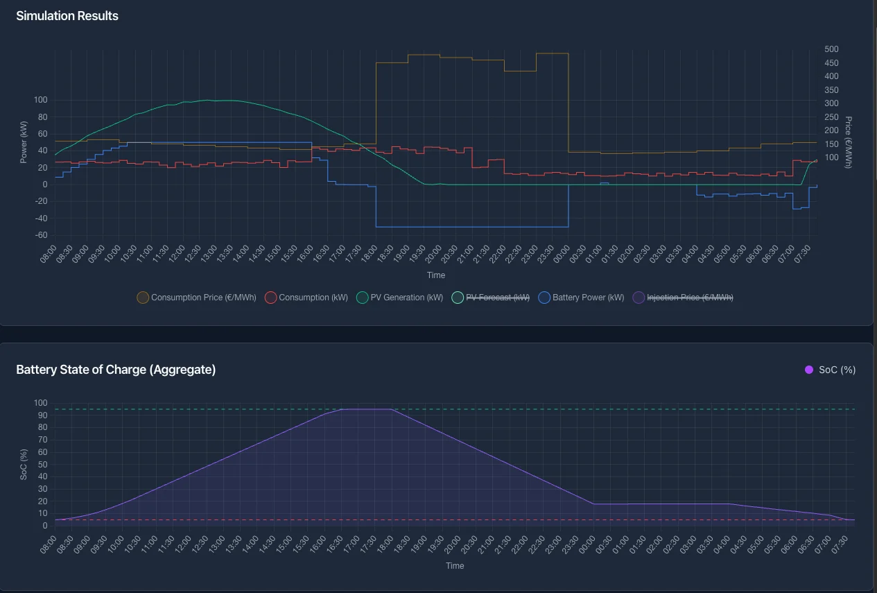
Cost optimization, evening high prices scenario — The algorithm charges during the cheap, sunny daytime and discharges into the expensive evening peak, buying low and using high. The chart is in English.

During the day the battery charges from cheap PV surplus, and in the evening peak it discharges to cover the expensive consumption. The full breakdown of this scenario is on the Battery schedule page.

Relationship to an external signal

Cost optimization is a local strategy. When an external signal partner is actively steering the installation, that partner takes precedence and cost optimization does not drive the battery. When no external signal is active, the battery follows the cost-optimization schedule. When the partner is on standby, so connected but not activating the battery, the battery idles and keeps its state of charge. A per-site option makes it follow the cost-optimization schedule during standby instead.